Exoplanets

Summary


Astrophysics research has never been more active. There are numerous fundamental questions being addressed, with big science missions to match. Because so much material is freely available to be analysed, it’s a wonderful time for citizen scientists.

Some key questions

  • formation of early universe

  • the dark sector

    • nature of dark energy

    • and of dark matter

  • the mysteries of our solar system

  • exoplanets

    • bio-signatures

    • techno-signatures

Where is all this information…

What’s happening in the field

  • mountain-top telescopes

  • space-based telescopes

  • radio-wave arrays

  • doing a lot of work in Infra-Red these days

  • spectroscopy

  • time-domain

Exoplanets

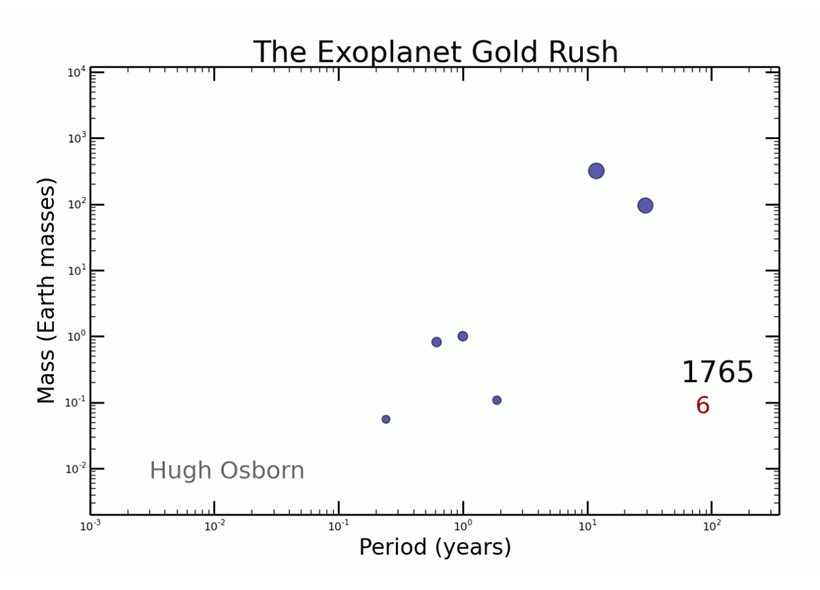
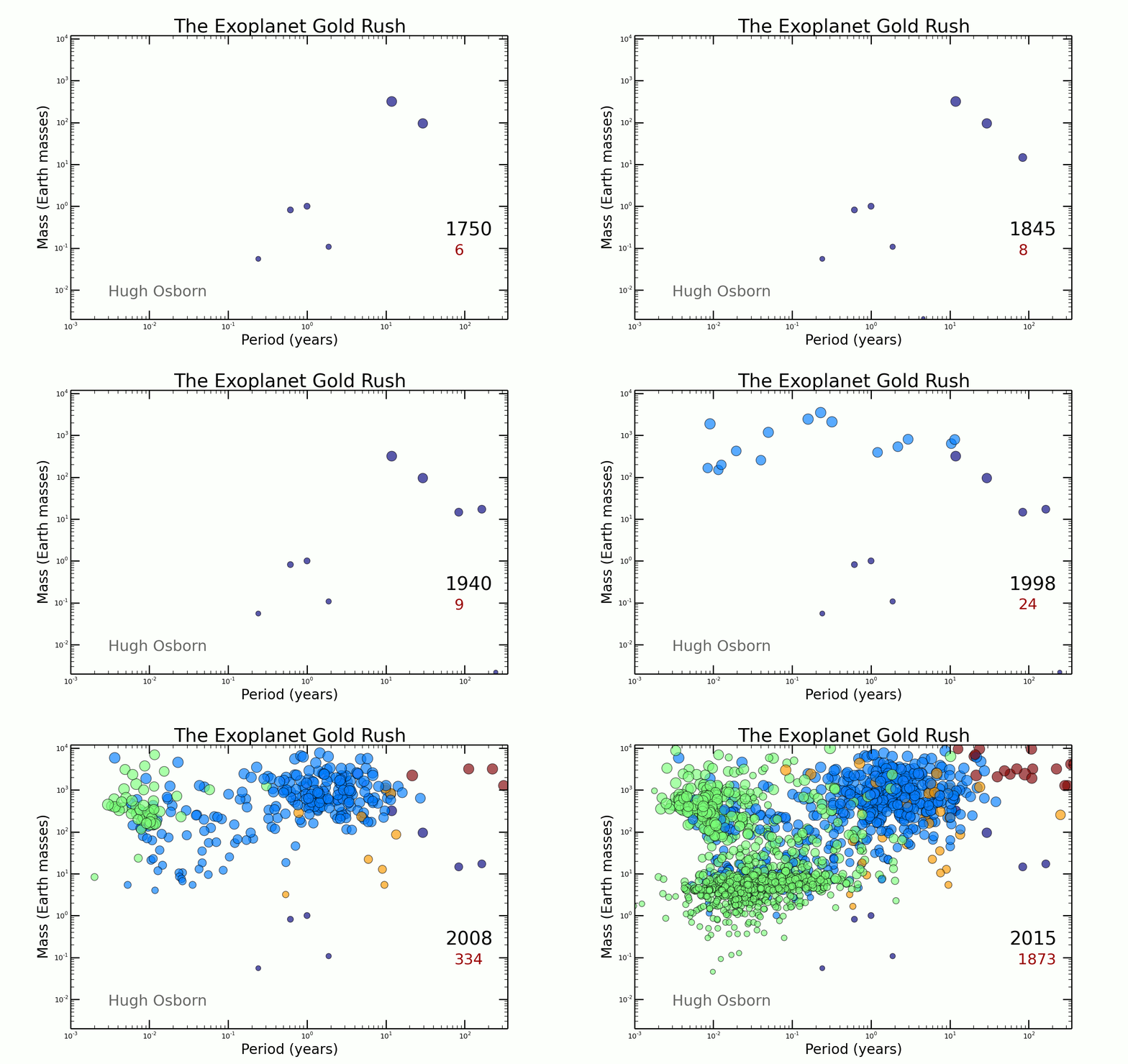
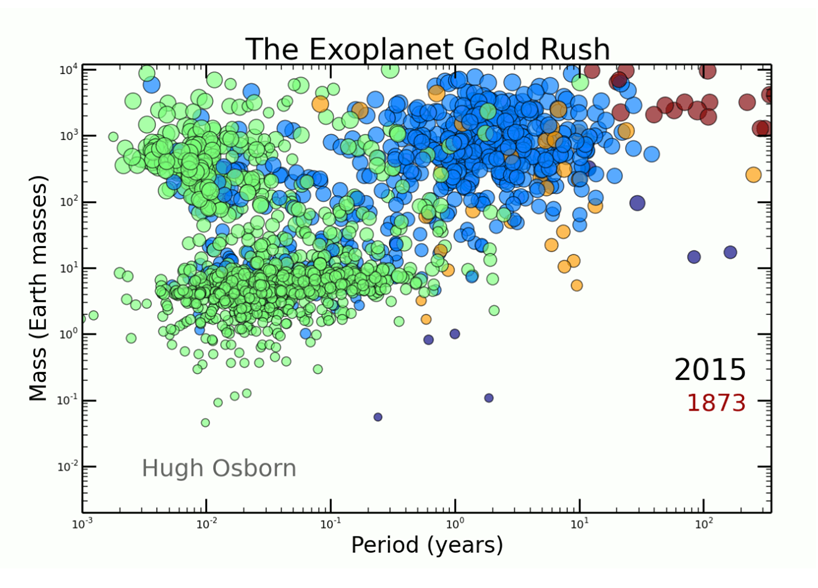
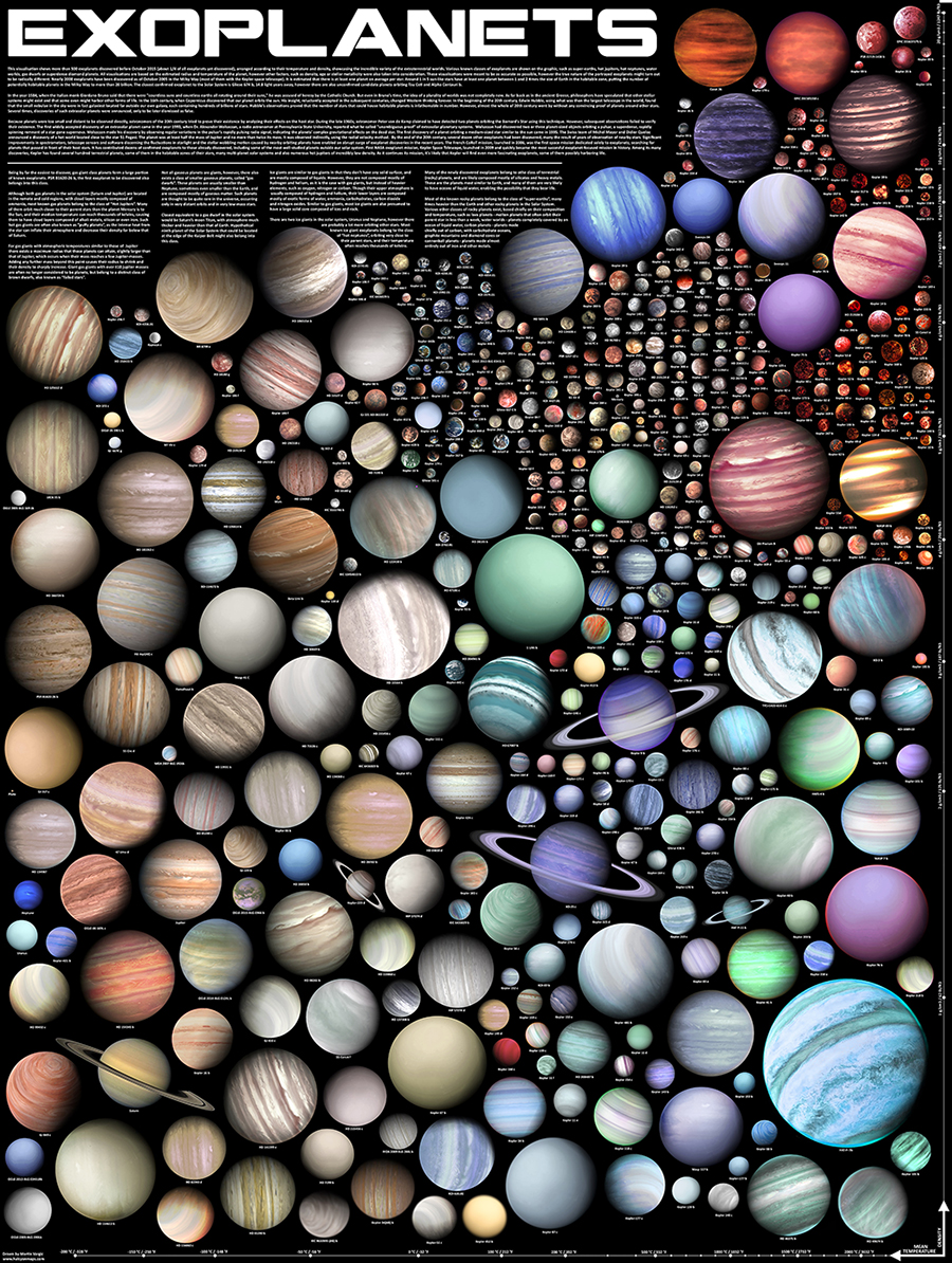
  • over 6000 confirmed

    • enough to do statistics

    • loads more candidates

      • pressing need for follow up studies
    • lots being discovered in legacy data

  • detect by:

    • transits - they pass in front of their host star making them a little dimmer

      • also, transit timing variations
    • radial velocity - the host star wobbles as the planet orbits, can be picked up by doppler shift in spectum

    • note, we never get to directly see the planet

Martin Vargic

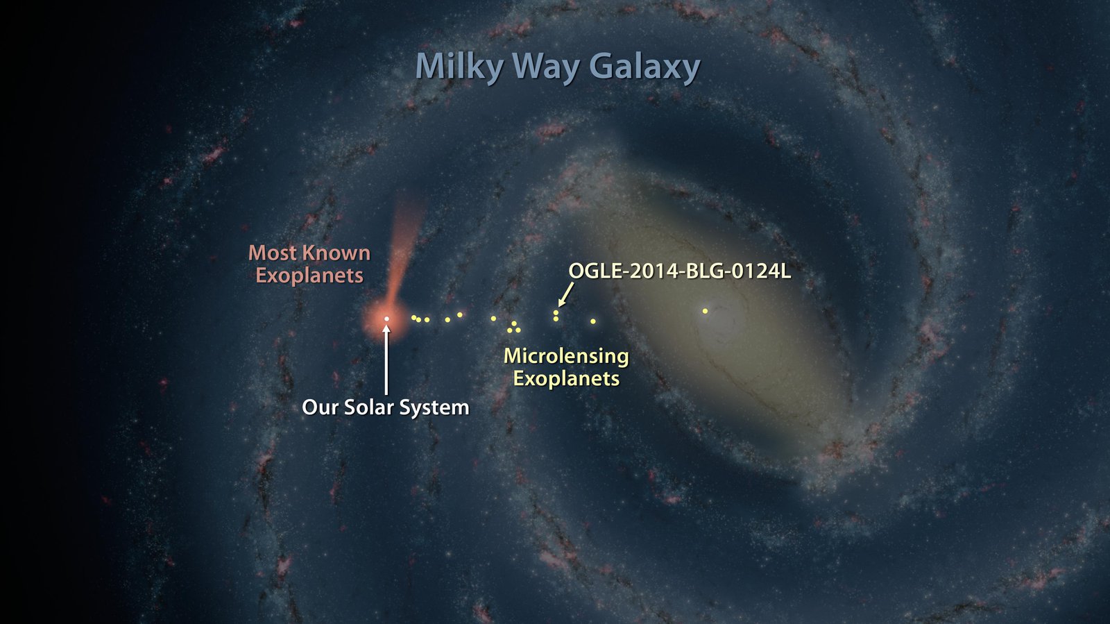
Where are they (so far)

Image from JPL

How to find them

  • radial velocity method

  • transit method

  • micro-lensing

  • transit timing variations

  • direct detection

Radial Velocity

  • as planet orbits, the star wobbles

  • not much as the star is so much more massive

    • our Sun does 500km wobble every year because of Earth’s orbit
  • if lined up properly, sometimes the star moves towards us, sometimes recedes

  • this movement will Doppler-shift the light from the star

  • we can detect this


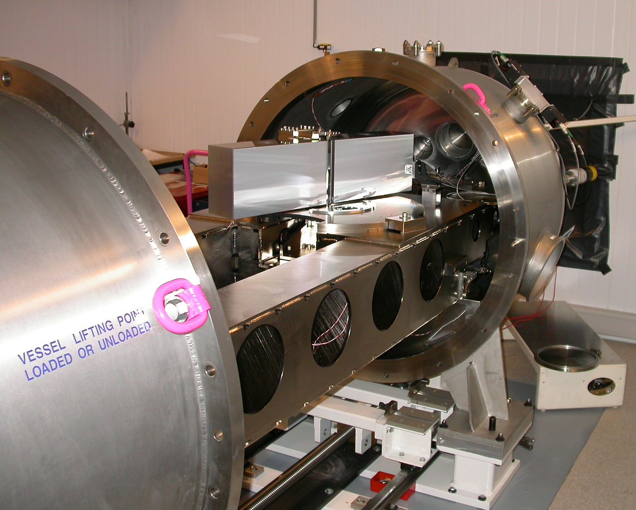
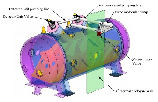
HARPS


ESPRESSO

What do we Know

  1. how far from its sun (from orbital period)

  2. measure planet size (how much dimming by transit)

  3. planet mass (from how much wobble it causes)

    • these last two give us planet density

    • can figure out if it’s a lump of rock or a ball of gas. And everything in between

  4. Starting to get spectra of exoplanet atmospheres

Surprises

  • they are so common, seems like default for a star to have planets

    • weren’t expecting this, thought they’d be rare
  • most systems have close in planets

    • we just have Mercury at 88 days
  • planets migrate

    • find planets in orbits where they couldn’t possibly have formed

    • c.f. hot Jupiters

  • beefed up version of Earth is by far most common type

    • nothing like this in our solar system
  • orbits aren’t very circular

  • beads-on-a-string mechanism quite common

What comes next

  • exoplanet spectra will be a big deal

    • what gasses are in the atmosphere

    • even isotope abundances (\(^{13}C / ^{12}C\) and \(^{18}O / ^{16}O\))

    • look for bio-signatures

    • look for techno-signatures

Our Work

  • most of the heavy lifting done from space (Kepler, TESS…..)

  • need ground based follow-up, or indeed discovery

    • possible with modest telescope
  • atmosphere is a big problem

    • differential photometry

    • if all stars vary simultaneously, it’s the atmosphere

    • if one blinks on its own, could be interesting

    • need good reference stars

      • same colour, similar intensity

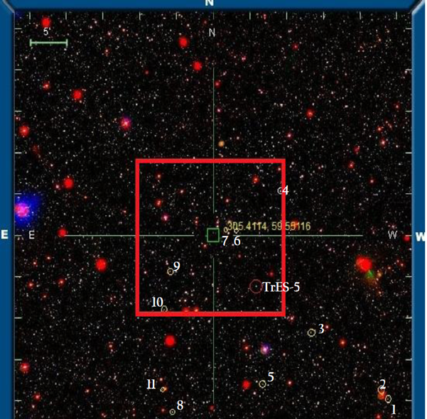
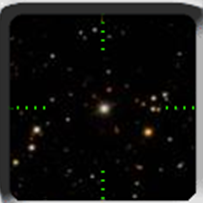
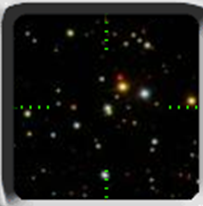
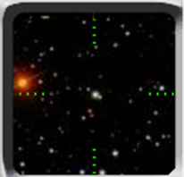
      • our job is identifying fields with hosts of clone stars

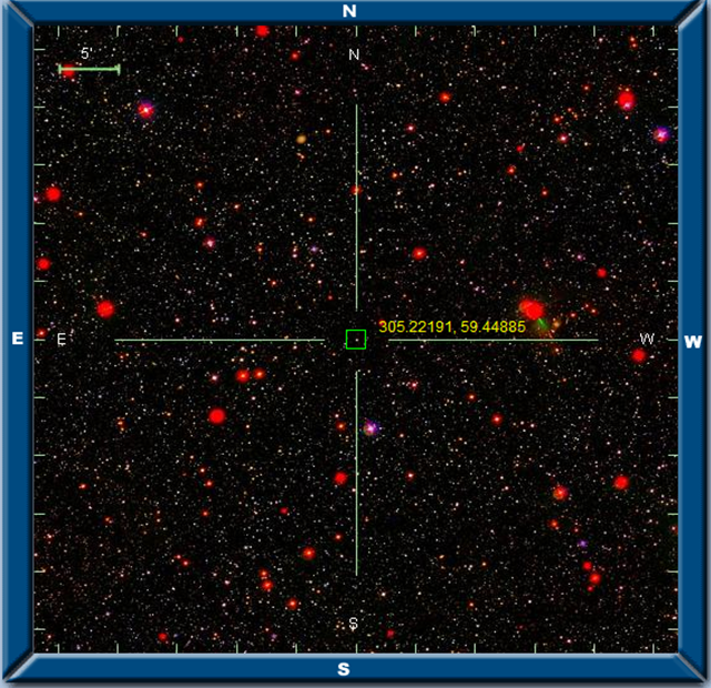
TrES-5

What makes a clone?

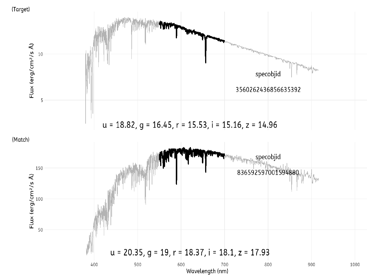
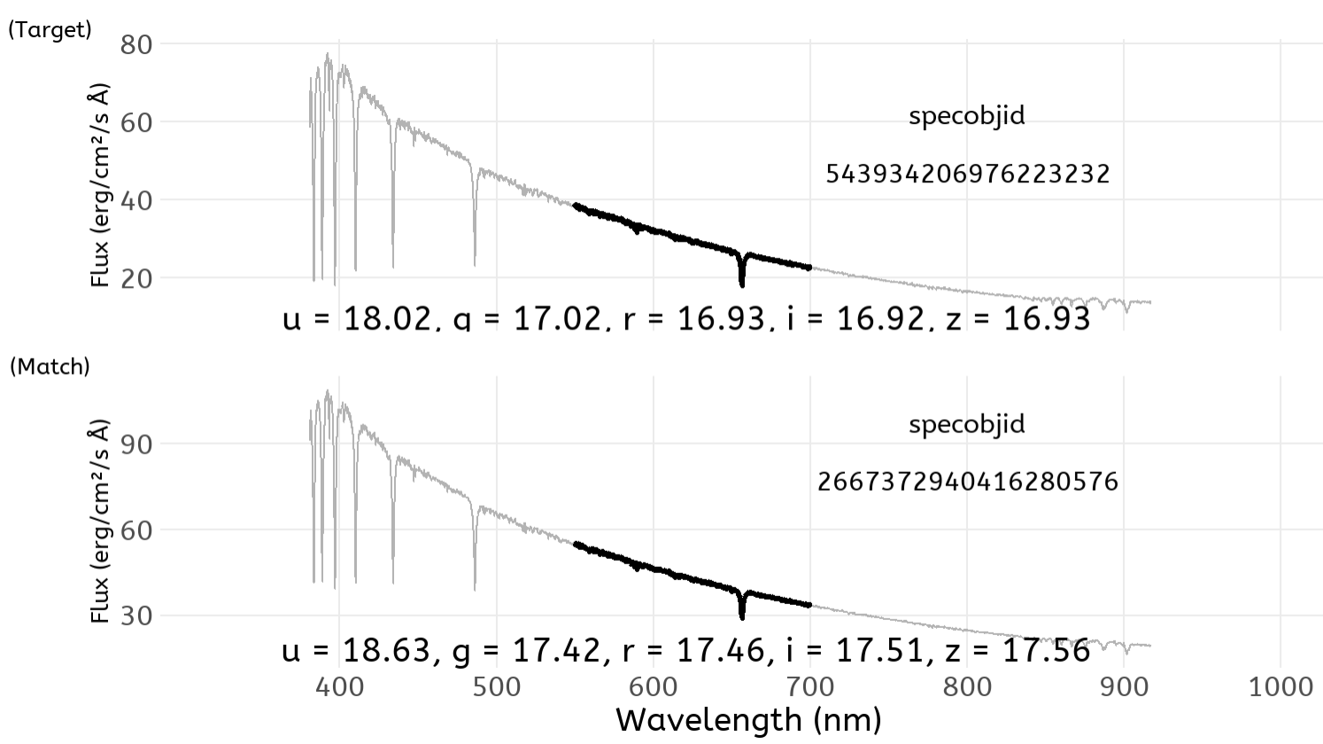
  • ideally stellar spectra should be the same

  • for most stars, don’t have a spectrum, just (5) colours in different wavelength bands

  • need some way to assess suitablity with this limited information

  • time for some machine learning

    • use stars with the full information

    • use them to infer behaviour for stars where we know less

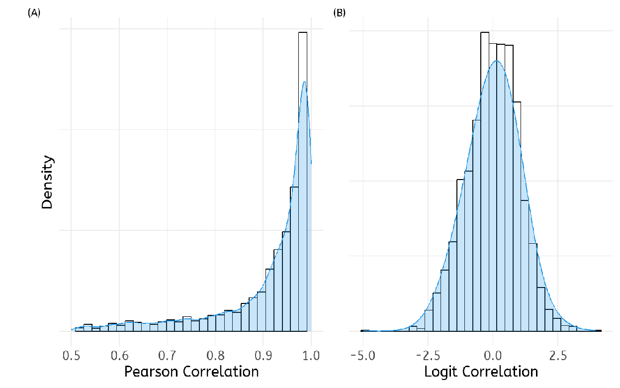
  • take correlation between spectra

    • but correlation always between -1 and +1

    • transform by logit()

      • \(logit(x) = log_e \frac{1+x}{1-x}\)

data handling

  • not hard to generate lots of data

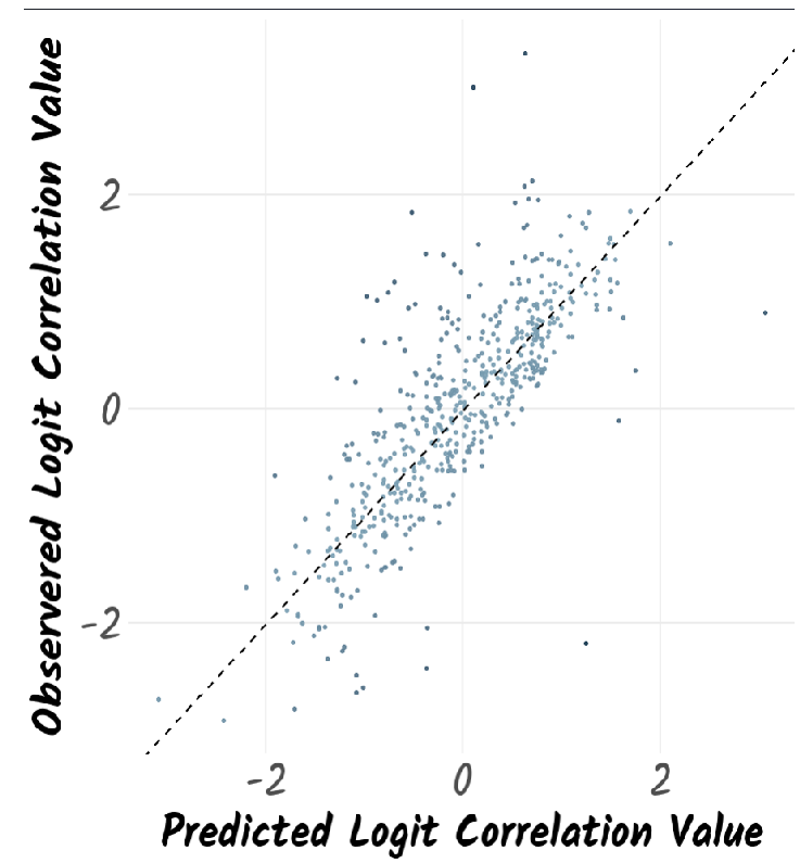
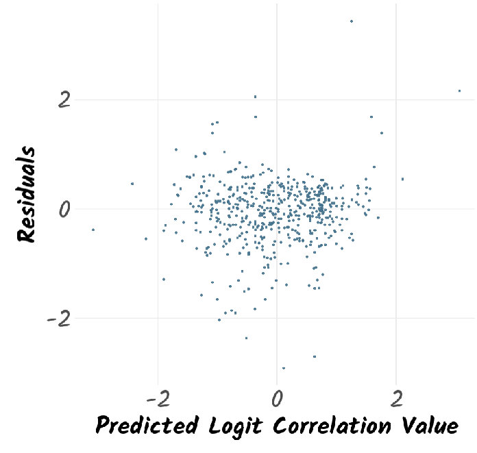
    • we settled for about 5000 pairs
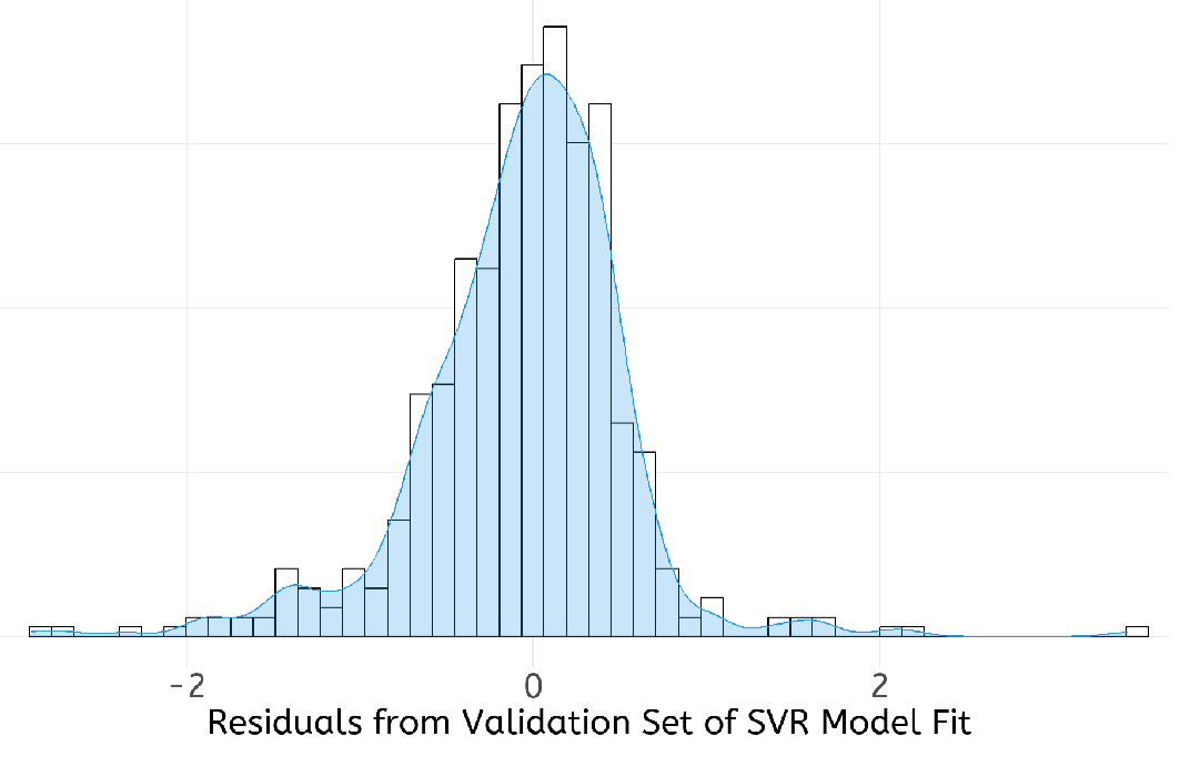
  • split into training (70%), test (15%), and validation (15%)

Modelling

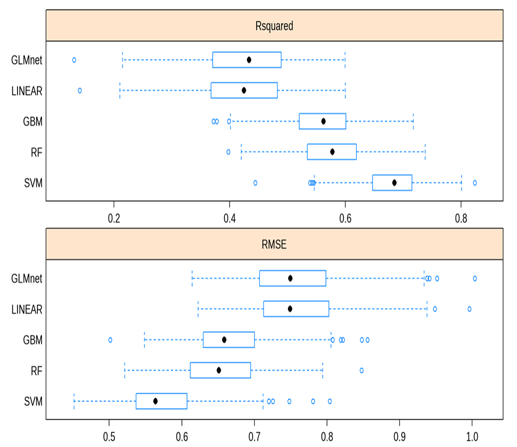
  • applied 5 models to our data

    • LM, RF, SVR, GBM, GLM
  • SVR did best

    • not surprising given nature of problem

  • Support Vector Regression follows the general principle of Support Vector Machines, but for regression rather than classification. It fits the data using a hyperplane, a plane in high dimensional space. An extra dimension is added using a kernel that facilitates fitting complex relationships. The hyperparameters Cost and 𝜎 are used to reduce overfitting of the data. The work here used a radial basis kernel function (Karatzoglou et al., 2004). A grid search on the hyperparameters Cost (C) and sigma (𝜎) was undertaken for values 8 < C < 25 and 0.08 < 𝜎 < 0.20. The model was optimised based on the RMSE of the training set. The best tune was obtained for C = 20 and 𝜎 = 0.12.

  • Random Forests consist of an ensemble of a large number of decision trees (Breiman, 2001). Each tree is built from different subsamples of the training data. In addition, the split at each node is chosen based on a random subset of features which differs at every split. For regression, the mean of the predicted value from every tree is taken to be the overall predicted value. The work here used the ranger fast implementation of random forests (Wright and Ziegler, 2017). The number of trees was set to 500. The Minimum Node Size was set to be 5, the splitting rule was chosen to be variance. The number of variables to possibly split at each node (mtry) was tuned to be 6.

  • Gradient Boosting uses an iterative series of decision trees where poorly predicted values in the training set are up-weighted in subsequent iterations. Here Friedman’s gradient boosting algorithm (Boehmke and Greenwell, 2019) was used. A grid search on the hyperparameters Number of Boosting Iterations (n.trees), Maximum Tree Depth (interaction.depth), Shrinkage (shrinkage) which corresponds to the Learning Rate, and Minimum Terminal Node Size (n.minobsinnode) was undertaken. The model was optimised based on the RMSE of the training set. The best tune was obtained for n.trees = 100, interaction.depth = 10, n.minobsinnode = 10, and shrinkage = 0.1.

  • Generalised Linear Model fits generalised linear models by optimising the maximum likelihood (Friedman et al., 2010). It implements regularisation via a hyperparameter 𝛼 that varies from 0 (ridge regression) to 1 (lasso regression). It also optimises a regularisation penalty, 𝜆. The best performing parameters here were 𝛼 = 0.1 and 𝜆 = 6.7×10⁻⁴

  • Linear Model was the simplest model used in this work. It consisted of refining an intercept as well as coefficients for each of the ten features in the model that minimised the RMSE between predicted and observed logit correlations. The linear model used the MASS R package (Venables and Ripley, 2002). There were no tunable parameters.

and now….

  • use this to point at stars

  • calculate benefit of the better reference stars