09-Hydrogen Atom

Physics Theory II PHYS2001

Summary

Expanding the Schrödinger Equation to 3 dimensions lets us have a look at problems such as the hydrogen atom. Because of the symmetry of the Coulomb potential, it makes sense to transform to spherical polar (\(r, \theta, \phi\)) rather than x, y, z. Separation of variables will lead to three equations, each of which will configure a quantum number for hydrogen.

We’ll then look at the available energy levels and thus the spectrum of hydrogen.

3-D Time Dependent Schrödinger Equation
Separation of Variables
Hydrogen Quantum Numbers
Hydrogen Wavefunctions
Bohr Radius
Hydrogen Spectrum
Hydrogen-Like Ions

3-D Time Independent Schrödinger Equation

in 3-D, Schrödinger looks like this:

\(- \frac{\hbar^2}{2m} (\frac{\partial ^2}{\partial x^2} + \frac{\partial ^2 }{\partial y^2} + \frac{\partial ^2 }{\partial z^2})\psi + V(x) \psi = E \psi\)

Hydrogen atom potential, V, due to electrostatic attraction of nucleus
This is spherically symmetrical, makes sense to switch to spherical polar coords
Time independent Shrödinger equations becomes

\({\displaystyle -{\frac {\hbar ^{2}}{2m }}\left[{\frac {1}{r^{2}}}{\frac {\partial }{\partial r}}\left(r^{2}{\frac {\partial \psi }{\partial r}}\right)+{\frac {1}{r^{2}\sin \theta }}{\frac {\partial }{\partial \theta }}\left(\sin \theta {\frac {\partial \psi }{\partial \theta }}\right)+{\frac {1}{r^{2}\sin ^{2}\theta }}{\frac {\partial ^{2}\psi }{\partial \varphi ^{2}}}\right]\\-{\frac {e^{2}}{4\pi \varepsilon _{0}r}}\psi =E\psi }\)

Assume that potential, V, just depends on r, not \(\theta\) or \(\phi\)
- True for hydrogen (or \(He^+\), \(Li^{++}\), \(Be^{3+}\)….)
- Pretty true for most ions and atoms
- Lousy for molecules
- We’ll see that the solution to

\({\displaystyle -{\frac {\hbar ^{2}}{2m }}\left[{\frac {1}{r^{2}}}{\frac {\partial }{\partial r}}\left(r^{2}{\frac {\partial \psi }{\partial r}}\right)+{\frac {1}{r^{2}\sin \theta }}{\frac {\partial }{\partial \theta }}\left(\sin \theta {\frac {\partial \psi }{\partial \theta }}\right)+{\frac {1}{r^{2}\sin ^{2}\theta }}{\frac {\partial ^{2}\psi }{\partial \varphi ^{2}}}\right] \\ -{\frac {e^{2}}{4\pi \varepsilon _{0}r}}\psi =E\psi }\)

gives us……

Separation of variables
Consider \(\psi(r, \theta, \phi) = R(r) Y(\theta, \phi)\)
Divide through by \(\psi\) and multiply by \(r^2\) to get
\(-\frac{\hbar^2}{2m} \frac{1}{R} \frac{\partial}{\partial r} \left( r^{2} \frac{\partial R}{\partial r} \right) + r^2V - r^2E = \\ \frac{\hbar^{2}}{2m} \frac{1}{Y} \frac{1}{\sin\theta} \frac{\partial}{\partial \theta} \sin \theta \frac{\partial Y}{\partial \theta} + \frac{\hbar^{2}}{2m} \frac{1}{Y} \frac{1}{\sin^2\theta} \frac {\partial ^{2}Y }{\partial \varphi ^{2}}\)

Left side just depends on r, right side just depends on \(\theta\) and \(\phi\)
Then they must both be equal to a constant
Let this equal \(-\lambda\), say
\(-\frac{\hbar^2}{2m} \frac{1}{R} \frac{d}{d r} \left( r^{2} \frac{d R}{d r} \right) + r^2V - r^2E = -\lambda\)
\(\frac{\hbar^{2}}{2m} \frac{1}{Y} \frac{1}{\sin\theta} \frac{\partial}{\partial \theta} \sin \theta \frac{\partial Y}{\partial \theta} + \frac{\hbar^{2}}{2m} \frac{1}{Y} \frac{1}{\sin^2\theta} \frac {\partial ^{2}Y }{\partial \varphi ^{2}} = -\lambda\)

Leave aside radial part for the moment
Further separate the angular terms
Put \(Y(\theta, \phi) = \Theta(\theta) \times \Phi(\phi)\)
Divide through by \(Y\) and multiply by \(\sin^2\theta\)
\(\frac{\hbar^{2}}{2m} \frac{\sin\theta}{\Theta} \frac{\partial}{\partial \theta} \sin\theta \frac{\partial\Theta }{\partial \theta} + \lambda \sin^2 \theta = -\frac{\hbar^{2}}{2m} \frac{1}{\Phi}\frac{\partial^2 \Phi}{\partial \phi^2}\)

Left hand side depends just on \(\theta\)
Right hand side depends just on \(\phi\)
Must both be equal to some constant, \(\nu\) say
\(\frac{\hbar^{2}}{2m} \frac{\sin\theta}{\Theta} \frac{d}{d \theta} \sin\theta \frac{d\Theta }{d \theta} + \lambda \sin^2 \theta = \nu\)
\(-\frac{\hbar^{2}}{2m} \frac{1}{\Phi}\frac{d^2 \Phi}{d \phi^2} = \nu\)
later on we’ll set \(\nu = \mathcal{l}(\mathcal{l} + 1)\) because the \(\mathcal{l}\) is related to angular momentum

\(\Phi\) part is easy
- \(-\frac{\hbar^{2}}{2m} \frac{1}{\Phi}\frac{d^2 \Phi}{d \phi^2} = \nu\)
- gives solution \(\Phi = A e ^{ \pm i \sqrt{\frac{2m\nu}{\hbar^2}} \phi }\)
this must be single valued so:
\(\Phi(\phi + 2\pi) = \Phi(\phi)\)

\(\implies e ^{ \pm i \sqrt{\frac{2m\nu}{\hbar^2}} 2\pi } = 1\)

\(\implies \sqrt{\frac{2m\nu}{\hbar^2}} = {\color{red}{m_{\mathcal{l}}}}\)
where \({\color{red}{m_{\mathcal{l}}}}\) is some integer; positive, negative, or zero

subbing back into \(\Phi\) we get
\(\Phi = \frac{1}{\sqrt{2\pi}} e^{i {\color{red}{m_{\mathcal{l}}}} \phi}\)
factor \(\frac{1}{\sqrt{2\pi}}\) is first step in normalising
we now have our first quantum number, \({\color{red}{m_{\mathcal{l}}}}\)

Solution for \(\Theta\) is more complex
Get Legendre polynomials
These are akin to Hermite polynomials we met with the SHO

The three separated equations are:

\(\frac{\hbar^2}{2m} \frac{1}{r^2} \frac{d}{d r} \left( r^{2} \frac{d R}{d r} \right) + \left[\frac{e^2}{4\pi\epsilon_0r} + E - \frac{\lambda}{r^2}\right]R = 0\)
\(\frac{\hbar^{2}}{2m} \frac{1}{\sin\theta} \frac{d}{d\theta} \sin\theta \frac{d\Theta }{d \theta} + \left[ \lambda - \frac{\nu}{\sin^2 \theta} \right]\Theta = 0\)
\(\frac{\hbar^{2}}{2m} \frac{d^2 \Phi}{d \phi^2} + \nu \Phi = 0\)

Each equation gives a quantum number

– the \(\Phi\) equation as we’ve seen gives \({\color{red}{m_{\mathcal{l}}}}\)
- This is the z component of angular momentum
- Called magnetic quantum number

– \(\Theta\) equation will give \(\mathcal{l}\) where \(\nu = \mathcal{l}(\mathcal{l} + 1)\)

where \(\mathcal{l}\) is related to the total angular momentum
Called orbital quantum number

– R equation gives n

Called principle quantum number
\(\Phi\) quantisation comes from need to be single valued
Other two come from truncating a polynomial

– otherwise wavefunction couldn’t be kept finite at large r

– We wouldn’t be able to normalise \(\psi\)

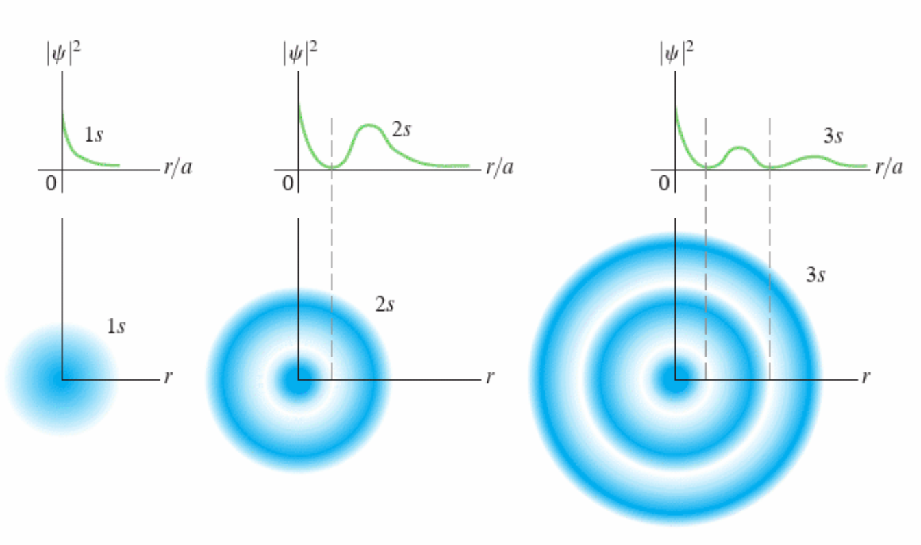
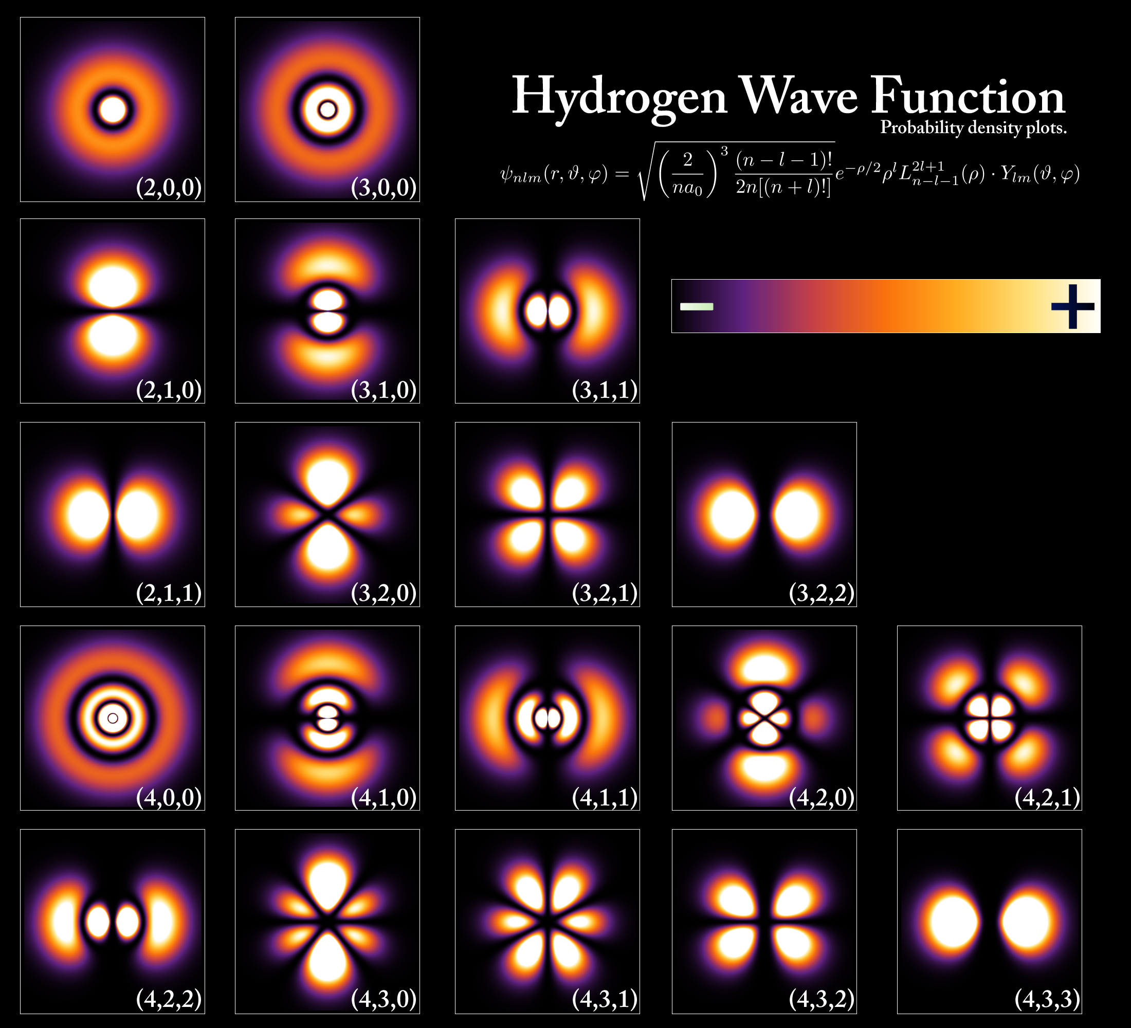
Some Hydrogen Wavefunctions

\({\color{purple}{Radial \; R(r)}}\), \({\color{darkgreen}{Polar \; \Theta(\theta)}}\), and \({\color{red}{Azimuthal \; \Phi(\phi)}}\)

\({\color{purple}{n=1}}\), \({\color{darkgreen}{\mathcal{l} = 0}}\), \({\color{red}{m_{\mathcal{l}} = 0}}\)
- \(\psi({\color{purple}{r=1}}, {\color{darkgreen}{\theta=0}}, {\color{red}{\phi=0}}) = {\color{purple}{\frac{2}{a_0^{3/2}} e^{-r/a_0}}} \times{\color{darkgreen}{\frac{1}{\sqrt{2}}}} \times {\color{red}{\frac{1}{\sqrt{2 \pi}}}}\)
\({\color{purple}{n=2}}\), \({\color{darkgreen}{\mathcal{l} = 0}}\), \({\color{red}{m_{\mathcal{l}} = 0}}\)
- \(\psi({\color{purple}{r}}, {\color{darkgreen}{\theta}}, {\color{red}{\phi}}) = {\color{purple}{\frac{1}{\sqrt{2} a_0^{3/2}} \left[1-\frac{r}{2a_0}\right] e^{-r/2a_0}}} \times{\color{darkgreen}{\frac{1}{\sqrt{2}}}} \times {\color{red}{\frac{1}{\sqrt{2 \pi}}}}\)
\({\color{purple}{n=3}}\), \({\color{darkgreen}{\mathcal{l} = 0}}\), \({\color{red}{m_{\mathcal{l}} = 0}}\)
- \(\psi({\color{purple}{r}}, {\color{darkgreen}{\theta}}, {\color{red}{\phi}}) = {\color{purple}{\frac{2}{81 \sqrt{3} a_0^{3/2}} \left[27-18\frac{r}{2a_0}+2(\frac{r}{2a_0})^2 \right] e^{-r/2a_0}}} \times{\color{darkgreen}{\frac{1}{\sqrt{2}}}} \times {\color{red}{\frac{1}{\sqrt{2 \pi}}}}\)

\({\color{purple}{Radial \; R(r)}}\), \({\color{darkgreen}{Polar \; \Theta(\theta)}}\), and \({\color{red}{Azimuthal \; \Phi(\phi)}}\)

\({\color{purple}{n=2}}\), \({\color{darkgreen}{\mathcal{l} = 1}}\), \({\color{red}{m_{\mathcal{l}} = 0}}\)
- \(\psi({\color{purple}{r}}, {\color{darkgreen}{\theta}}, {\color{red}{\phi}}) = {\color{purple}{\frac{1}{\sqrt{6} a_0^{3/2}} \frac{r}{2a_0} e^{-r/2a_0}}} \times{\color{darkgreen}{\frac{\sqrt{6}}{2} \cos \theta}} \times {\color{red}{\frac{1}{\sqrt{2 \pi}}}}\)
\({\color{purple}{n=2}}\), \({\color{darkgreen}{\mathcal{l} = 1}}\), \({\color{red}{m_{\mathcal{l}} = \pm 1}}\)
- \(\psi({\color{purple}{r}}, {\color{darkgreen}{\theta}}, {\color{red}{\phi}}) = {\color{purple}{\frac{1}{\sqrt{6} a_0^{3/2}} \frac{r}{2a_0} e^{-r/2a_0}}} \times{\color{darkgreen}{\frac{\sqrt{3}}{2} \cos \theta}} \times {\color{red}{\frac{1}{\sqrt{2 \pi}} e^{\pm i \phi} }}\)

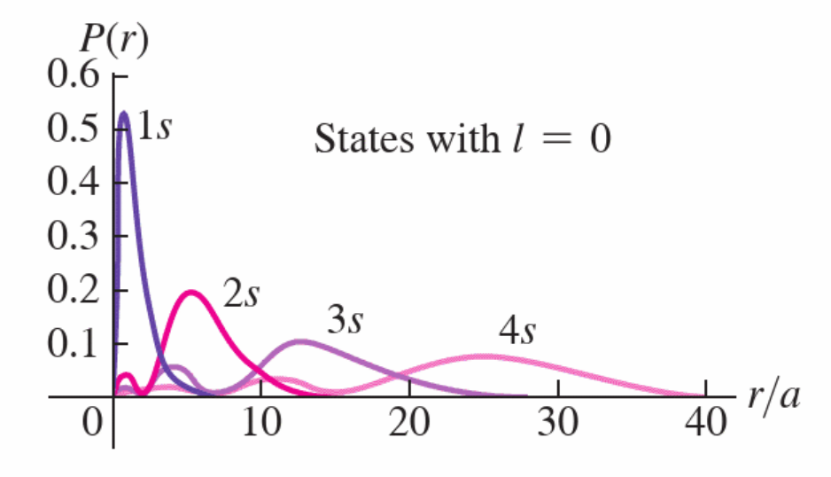
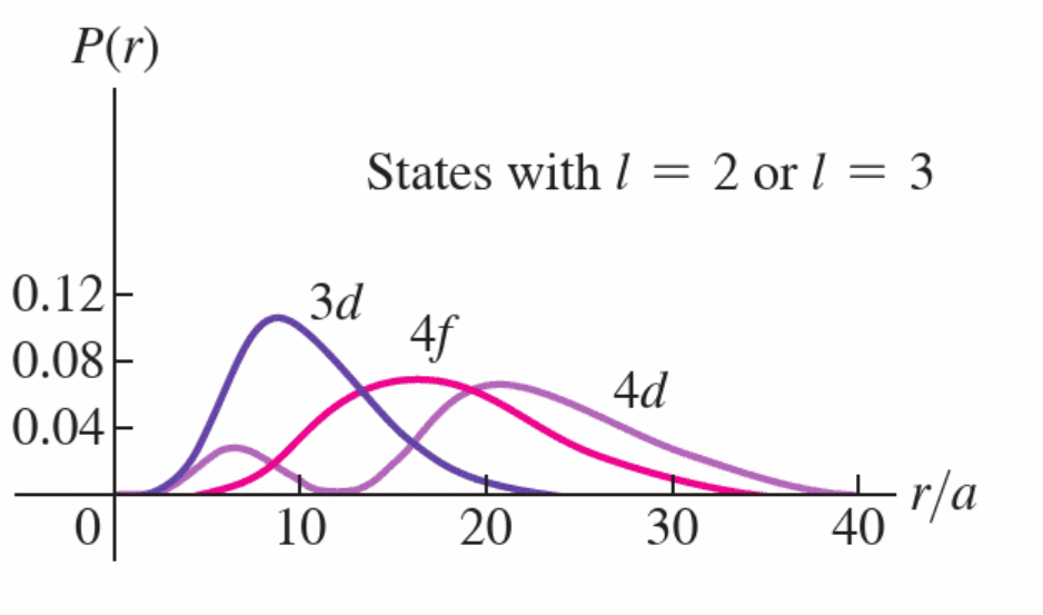
\(a_0\) is the Bohr Radius

in the equations above used \(a_0 = \frac{4 \pi \epsilon_0 \hbar^2}{e^2m} = 0.0529nm\)
this is the Bohr Radius
corresponds to most likely distance from nucleus for electron when \(n=1\)

Young & Freedman

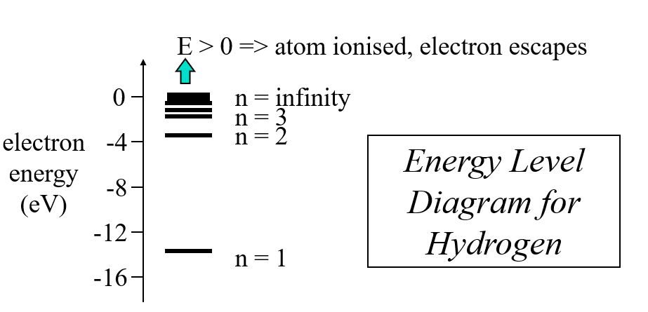
Principle Quantum Number, n, and Energy Levels in Hydrogen

electrostatic energy in Hydrogen only depends on how far you are from the nucleus
- radial part, \(R(r)\), is only bit which matters
- no dependence on \(\Theta(\theta)\) or on \(\Phi(\phi)\)
- values of \({\mathcal{l}}\) and \({m_{\mathcal{l}}}\) are degenerate

get \(E_n = -\frac{1}{(4\pi\epsilon_0)^2} \frac{me^4}{2 \hbar^2} \frac{1}{n^2}\)
this is (coincidentally) the same as the expression that Bohr got from his model
reduces to \(E_n = -\frac{13.6057}{n^2} eV\)

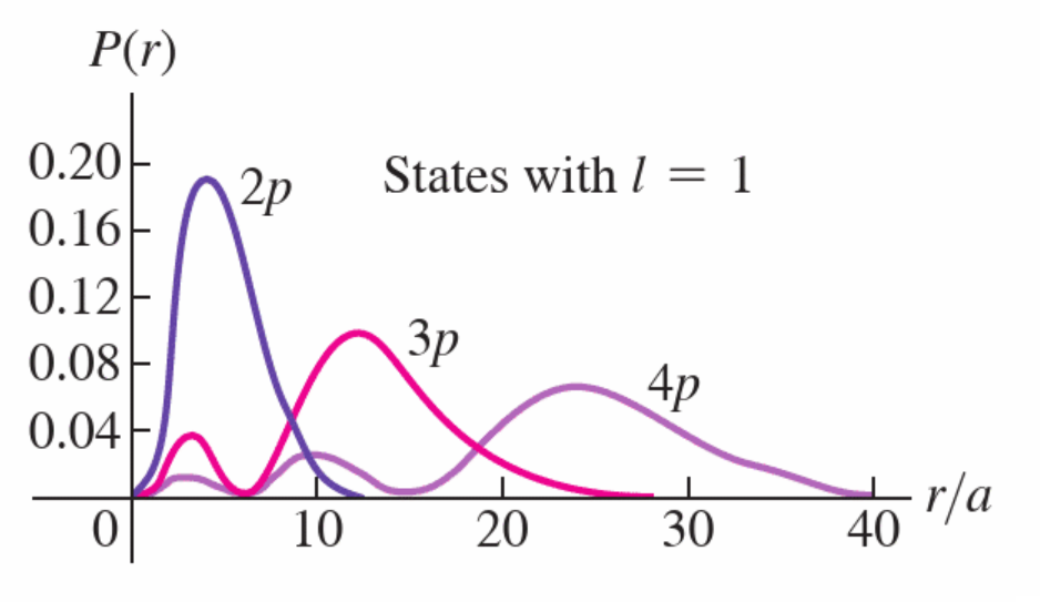
Orbital Quantum Number, \({\mathcal{l}}\), and Angular Momentum

the orbital angular momentum, \(L\) is given by:
\(L = \sqrt{{\mathcal{l}}({\mathcal{l}} + 1)}\hbar\) where \({\mathcal{l}} = 0, 1, 2...n-1\)
note the \({\mathcal{l}}\) can be 0 leading to zero angular momentum. Unlike simple picture of hydrogen, the electron isn’t orbiting around the nucleus

Magnetic Quantum Number, \(m_{\mathcal{l}}\), and Z-Component of Angular Momentum

\(m_{\mathcal{l}}\) dictates, kind of, the direction of the angular momentum, \(L\).
\(L_z = m_{\mathcal{l}}\hbar\) where \(m_{\mathcal{l}} = 0, \pm1, \pm2..., \pm {\mathcal{l}}\)
\(L_z\) is always less that \(L\), for obvious reasons
fact that \(L_z < L\) is consistent with uncertainty principle

wikipedia

Hydrogen Spectra

energy levels given by: \(E_n = -\frac{13.6057}{n^2} eV\)

transitions between levels lead to lines in the hydrogen spectrum

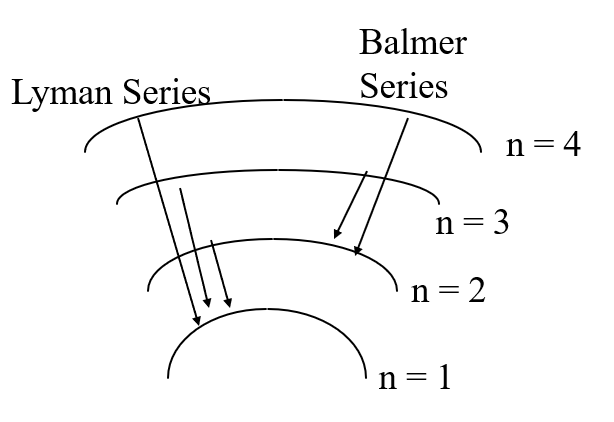
corresponding wavelengths for the photon emitted by each transition is given by
\(\frac{1}{\lambda} = \frac{1}{(4\pi\epsilon_0)^2} \frac{me^4}{4\pi \hbar^3 c} \left(\frac{1}{n_{low}^2} - \frac{1}{n_{high}^2}\right)\)
\(R = \frac{1}{(4\pi\epsilon_0)^2} \frac{me^4}{4 \pi \hbar^3 c} = 1.0974 \times 10^7 m^{-1}\)
R is the Rydberg Constant
get lines at 656nm, 486nm, 434nm, and 410nm in the visible.
- all Balmer series
- \(n_{low} = 2\)

Hydrogen-Like Ions

for hydrogen-like ions (\(He^+\), \(Li^{++}\), \(Be^{3+}\)), need extra factor of \(Z^2\) in energy levels
\(E_n = -\frac{1}{(4\pi\epsilon_0)^2} \frac{mZ^2e^4}{2 \hbar^2} \frac{1}{n^2}\)
\(E_n = - Z^2 \frac{13.6057}{n^2} eV\)
also need to modify Bohr Radius for these ions:
- \(a_0 = \frac{4 \pi \epsilon_0 \hbar^2}{Ze^2m} = \frac{0.0529}{Z} nm\)
- gives ground state wavefunction of \(\psi_0(r) = Ae^{-Zr/a_0}\)

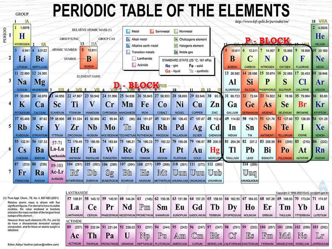
Back to Our Periodic Table

Principle quantum number, \(n\) gives level of orbital
The Orbital Quantum Number, \({\mathcal{l}}\), gives s, p, d, f etc
- 1s orbital has \(n=1\) and \({\mathcal{l}} = 0\)
- 2s orbital has \(n=2\) and \({\mathcal{l}} = 0\)
- 2p orbital has \(n=2\) and \({\mathcal{l}} = 1\)
- 3d orbital has \(n=3\) and \({\mathcal{l}} = 2\)
maximum number of electrons in each orbital given by number of posssible \(m_{\mathcal{l}}\) values \(\times 2\)
- max. no. = \((2 \times {\mathcal{l}} + 1) \times 2\)

Equations

\(- \frac{\hbar^2}{2m} (\frac{\partial ^2}{\partial x^2} + \frac{\partial ^2 }{\partial y^2} + \frac{\partial ^2 }{\partial z^2})\psi + V(x) \psi = E \psi\)

\(a_0 = \frac{4 \pi \epsilon_0 \hbar^2}{e^2m} = 0.0529nm\)
\(L = \sqrt{{\mathcal{l}} ({\mathcal{l}} + 1)}\hbar\)
\(L_z = m_{\mathcal{l}}\hbar\)
\(E_n = -\frac{1}{(4\pi\epsilon_0)^2} \frac{me^4}{2 \hbar^2} \frac{1}{n^2} \\ = -\frac{13.6057}{n^2} eV\)
\(\frac{1}{\lambda} = \frac{1}{(4\pi\epsilon_0)^2} \frac{me^4}{4\pi \hbar^3 c} \left(\frac{1}{n_{low}^2} - \frac{1}{n_{high}^2}\right)\)
\(R = \frac{1}{(4\pi\epsilon_0)^2} \frac{me^4}{4 \pi \hbar^3 c} = 1.0974 \times 10^7 m^{-1}\)

\(E_n = -\frac{1}{(4\pi\epsilon_0)^2} \frac{mZ^2e^4}{2 \hbar^2} \frac{1}{n^2} \\ = - Z^2 \frac{13.6057}{n^2} eV\)
\(a_0 = \frac{4 \pi \epsilon_0 \hbar^2}{Ze^2m} = \frac{0.0529}{Z} nm\)
\(\psi({\color{purple}{1}}, {\color{darkgreen}{0}}, {\color{red}{0}}) = {\color{purple}{\frac{2}{a_0^{3/2}} e^{-r/a_0}}} \times{\color{darkgreen}{\frac{1}{\sqrt{2}}}} \times {\color{red}{\frac{1}{\sqrt{2 \pi}}}}\)