08-Shrodinger Equation
Simple Harmonic Oscillator

Physics Theory II PHYS2001

Summary

For the next application of the Schrödinger Equation, we’ll look at a particle undergoing simple harmonic motion (SHO). This particle is in a parabolic potential and classically exhibits the kind of motion typical of pendula or stretched springs. This is typical of vibrational modes in molecules.

Wavefunctions revisited
The SHO potential
Hermite polynomials
SHO energy levels
Applications
Equations
References

Properties of Wavefunctions

the Schrödinger Equation is just a differential equation
various solutions depend on:
- the potential \(V(x)\)
- the boundary conditions
  - these lead to quantisation
in general, get a family of solutions with different \(\psi_n\) corresponding to different \(E_n\)
write \(\frac{\hbar^2}{2m} \frac{d ^2 \psi}{d x^2} + V(x) \psi = E\psi\) \(\implies H \psi = E \psi\) where \(H\) is the Hamiltonian

\(\psi_n\) is normalisable (Hilbert space)
- \(\int_{-\infty}^{+\infty} \psi_n(x)^2 dx = 1\)
(assumes real valued \(\psi\), otherwise \(\int_{-\infty}^{+\infty} \psi_n^*(x) \psi_n(x) dx = 1\))

the \(\psi_n\)’s are orthogonal
- \(\int_{-\infty}^{+\infty} \psi_n \psi_m dx = 0\)
- form a basis set
  - \(g(x) = \Sigma_{n=0}^\infty a_n \psi_n\)

operators

\(\psi(x)\) carries all the information we can get about measurements we’ll get on the particle
- \(\bar{x} = \int_{-\infty}^{+\infty} \psi_n(x) x \psi_n(x) dx\) gives average particle position
- \(\bar{x^2} = \int_{-\infty}^{+\infty} \psi_n(x) x^2 \psi_n(x) dx\) gives average of position squared
- \(\sqrt{\bar{x}^2 - \bar{x^2}}\) = spread of particle position
- \(-i\hbar \int_{-\infty}^{+\infty} \psi_n(x) \frac{d}{d x} \psi_n(x) dx = \vec{p_x}\) gives particle momentum
- \(-i\hbar \int_{-\infty}^{+\infty} \psi_n(x) (y \frac{d}{d z} - z \frac{d}{d y}) \psi_n(x) dx = \vec{L_x}\) gives particle angular momentum

Simple Harmonic Oscillator (SHO)

Something like a pendulum
- a system rocking back and forth about an equilibrium position
- Obeys Hooke’s Law: \(F=-kx\)
- Has elastic energies \(V(x) = ½ kx^2 = ½ m \omega ^2x^2\)
- \(\omega = \sqrt{k/m}\) is the angular velocity \(= 2 \pi f\)
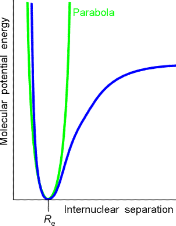
- Important in analysis of molecular vibrations
- Molecular bond not quite a simple harmonic system but good approximation for small vibrations
- Can look at departures from the ideal
  - Anharmonic terms
  - Perturbation theory (later on in course)

Apply Schrödinger Equation

\(- \frac{\hbar^2}{2m} \frac{d ^2 \psi}{d ^2} + V \psi = E\psi\)

\(V = \frac{1}{2} m \omega^2 x^2\)

\(\implies - \frac{\hbar^2}{2m} \frac{d ^2 \psi}{d x^2} + \frac{1}{2} m \omega^2 x^2 \psi = E\psi\)

To be normalisable, need a solution for \(\psi\) that goes to zero as x goes to \(\infty\)
try: \(\psi(x) = C e^{\frac{- \alpha x^2}{2}}\) where \(\alpha = \frac{m \omega}{\hbar}\)

Putting back into our Schrödinger Equation and equating powers of x we get:
- \(\alpha = \sqrt{\frac{mk}{\hbar^2}}\)
- \(E = ½ \hbar \omega\)
This is first of a series of solutions given by the general formula:
- \(\psi(x) = N_{\nu} H_{\nu}(x) e^{\frac{- \alpha x^2}{2}}\)
- role of \(N_{\nu}\) is to normalise wavefunction
  - \(N_{\nu} = \sqrt{\frac{1}{2^{\nu} \nu ! \sqrt{\pi}}}\)

Hermite Polynomials

\(H_{\nu}(x)\) are the Hermite Polynomials

\(H_0(x) = 1\)
\(H_1(x) = 2x\)
\(H_2(x) = -2 + 4x^2\)

\(H_3(x) = -12x + 8x^3\)
\(H_{\nu}(x) = (-1)^{\nu} e^{x^2} \frac{d^{\nu}}{dx^{\nu}} e^{-x^2}\)

SHO Energy Levels

gives family of energy levels given by \(E_n = (n + \frac{1}{2})\hbar \omega\)

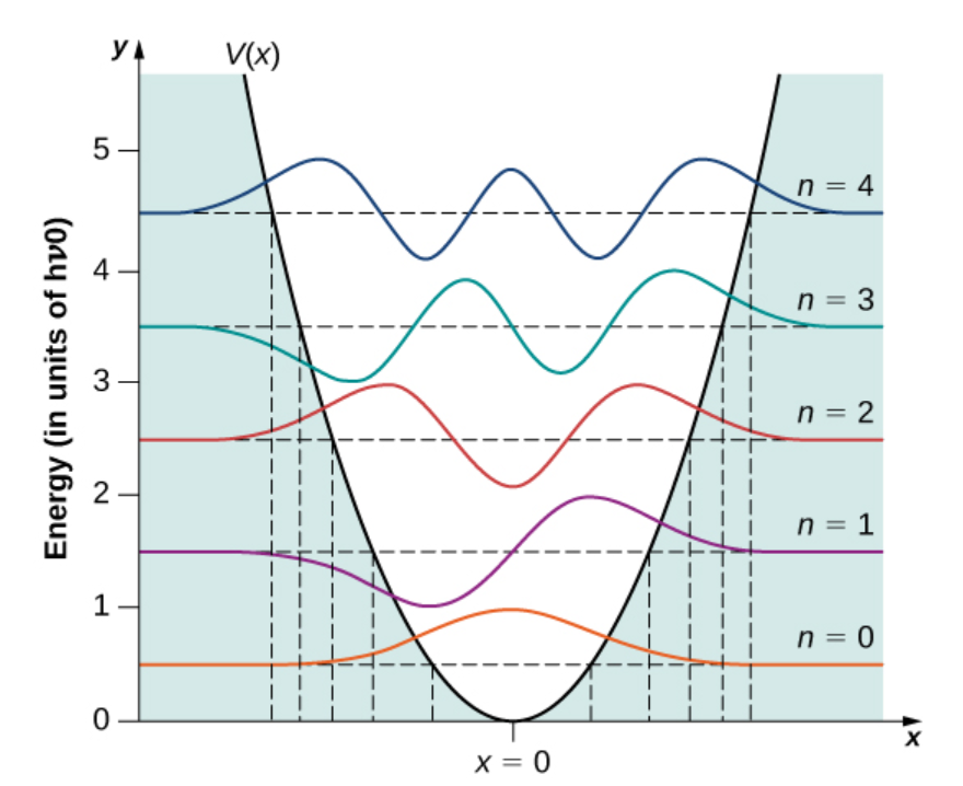
from openstax

Energy levels evenly spaced, separation \(= \hbar \omega\)
Lowest possible energy is not zero, it’s \(½\hbar \omega\)
- By the way, this is consistent with uncertainty principle
Quantum harmonic oscillator can stretch to extents that, classically, wouldn’t be allowed
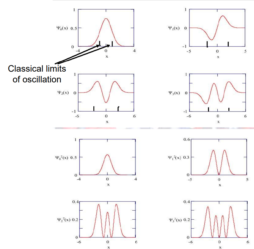
As the quantum number, \(n\), gets bigger and bigger the wavefunction starts to look more like classical case

– See wavefunctions on next page

Example

The strongest infrared band in CO occurs at \(2143cm^{-1}\). Find the force constant, \(k=m \omega^2\) for the C=O bond (m is the reduced mass, \(m = \frac{m_1m_2}{m_1 + m_2}\)) where \(m_1\) and \(m_2\) are the masses of an ion of carbon and of oxygen (\(m_{oxygen} = 2.66 \times 10^{-26}kg\) and \(m_{carbon} = 1.99 \times 10^{-26}kg\))
from \(E = \frac{hc}{\lambda}\) we get:
- \(E = 2143 \times 1.988 \times 10^{-23} = 4.26 \times 10^{-20}J\)
from \(E = \hbar \omega\) we get:
- \(\omega = \frac{4.26 \times 10^{-20}}{6.626 \times 10^{-34}} = 6.43 \times 10^{13} rads/s\)
from \(m = \frac{m_1m_2}{m_1 + m_2}\) we get:
- \(m = \frac{2.66 \times 10^{-26} \times 1.99 \times 10^{-26}}{2.66 \times 10^{-26} + 1.99 \times 10^{-26}} = 1.14 \times 10^{-26}kg\)
finally \(k=m \omega^2 = 1.14 \times 10^{-26} \times (6.43 \times 10^{13})^2 = 47.13\:N/m\)

Ladder Operators

Schrödinger Equation is \(\frac{\hbar^2}{2m} \frac{d ^2 \psi}{d x^2} + \frac{1}{2} m \omega^2 x^2 \psi = E\psi\)
rearrange: \(\frac{1}{2m} \left( (\frac{\hbar}{i}\frac {d}{d x})^2 + (m \omega x)^2 \right)\psi = E\psi\)
looks like a difference of squares; \(u^2 + v^2 = (u-iv)(u+iv)\)
- not quite, as here we have operators, not values
\(a_{\pm} = \frac{1}{\sqrt{2m}}(\frac{\hbar}{i} \frac{d}{dx} \pm im\omega x)\)
get \(a_- a_+ = \frac{1}{2m} \left( (\frac{\hbar}{i}\frac {d}{d x})^2 + (m \omega x)^2 \right) + \frac{1}{2}\hbar \omega\)

-ordering matters

\(a_+ a_- = \frac{1}{2m} \left( (\frac{\hbar}{i}\frac {d}{d x})^2 + (m \omega x)^2 \right) - \frac{1}{2}\hbar \omega\)
looking back at our Schrödinger Equation:
\((a_+ a_- + \frac{1}{2}\hbar \omega) \psi = E \psi\)
can show \(a_+ \psi_n\) satisfies the SE with energy \(E_n + \hbar \omega\)
likewise \(a_- \psi_n\) satisfies the SE with energy \(E_n - \hbar \omega\)

Equations

\(\frac{\hbar^2}{2m} \frac{d ^2 \psi}{d x^2} + \frac{1}{2} m \omega^2 x^2 \psi = E\psi\)
\(V(x) = ½ kx^2 = ½ m \omega ^2x^2\)
\(\omega = \sqrt{k/m} = 2 \pi f\)
\(\psi_0(x) = C e^{\frac{- \alpha x^2}{2}}\)
\(\alpha = \frac{m \omega}{\hbar} = \sqrt{\frac{mk}{\hbar^2}}\)

\(\psi(x) = N_{\nu} H_{\nu}(x) e^{\frac{- \alpha x^2}{2}}\)
\(N_{\nu} = \sqrt{\frac{1}{2^{\nu} \nu ! \sqrt{\pi}}}\)
\(H_{\nu}(x) = (-1)^{\nu} e^{x^2} \frac{d^{\nu}}{dx^{\nu}} e^{-x^2}\)
\(E_{\nu} = (\nu + \frac{1}{2})\hbar \omega\)

08-Shrodinger Equation Simple Harmonic Oscillator