07-Shrodinger Equation
Particle in a Box

Physics Theory II PHYS2001

eugene.hickey@tudublin.ie

Technological University Dublin

Summary

In our first application of the Schrödinger Equation, we’ll look at a particle in a 1 -dimensional box. This particle is at zero potential in the interval \(0 \leq x \leq a\) but cannot move outside these bounds.

Contents

1. Time Dependent Schrödinger Equation
2. Separation of Variables
   1. Time Independent Schrödinger Equation
3. Boundary Conditions

4. Nature of solutions
   • linearity
   • orthonormal
   • basis set
5. Square Examples
   • conjugated dyes
   • butadiene
6. Selection Rules

Time Dependent Schrödinger Equation

• finished last week with the Time Dependent Schrödinger Equation

\(i \hbar \frac{\partial \Psi}{\partial t} = - \frac{\hbar^2}{2m} \frac{\partial ^2 \Psi}{\partial x^2} + V\Psi\)

• Lots of times the potential, V, doesn’t depend on time, just position.

• There’s a neat trick called separation of variables we can use now.

\(\Psi (x, t) = \psi (x) T(t)\)

• Get:

\(i \hbar \frac{1}{T} \frac{\partial T}{\partial t} = - \frac{1}{\psi} \frac{\hbar^2}{2m} \frac{\partial ^2 \psi}{\partial x^2} + V(x)\)

• Left hand side just depends on time, right hand side just on x

\(\implies\) both sides must be equal to some constant, call it E say

\(\implies\) got ourselves two equations here

Time Dependence

• Working with the left (time) side of the equation gives us:

\(i \hbar \frac{d T}{d t} = E \times T(t)\)

• Solutions to this are fairly straightforward and not that interesting

\(T(t) = A e^{-iEt/\hbar}\)

• Gives temporal oscillations of the wavefunction

Time Independent Schrödinger Equation

• On the other hand, the spatial element is rich in solutions, depends on shape of V(x)

• Get

\(- \frac{\hbar^2}{2m} \frac{d ^2 \psi}{d x^2} + V(x) \psi = E \psi\)

• This is the time independent Schrödinger Equation

• Turns out, when we compare to the free space version, that E is the total energy of the system.

Boundary Conditions

• Solving problems using Time independent Schrödinger Equation means

  • Applying different natures of the potential, V

  • But also using boundary conditions, constraints on the wavefunction that tell us about the possible solutions

    • Wavefunction must be a continuous single valued function of position and time

    • The integral of the squared value of the wavefunction over all values of x must be finite (normalisable)

    • The first derivatives of the wavefunction in x must be continuous everywhere except when there is an infinite discontinuity in the potential

• We’ll first look at the nature of solutions to Schrödinger’s Equation, and then tackle some examples and put Schrödinger to work

Solutions of Schrödinger’s Equation

• Equation is linear in \(\psi\)

  • Superposition principle, if \(\psi_1\) and \(\psi_2\) are solutions then so is \(\psi_1 + \psi_2\)

    • and indeed \(A\psi_1 + B\psi_2\)

• Solution solved by eigenfunctions, \(\psi_n\), and corresponding eigenvalues, \(E_n\)

• Set of all solutions forms an orthogonal basis set

  • \(\int \psi_n \psi_m dx = 0 \;if \; n \neq m\)

  • Can make up any function from linear combination of \(\psi\)’s

    • \(F(x) = \Sigma \psi_n\)

Examples of Time Independent Schrödinger Equation

• Infinite square well

• Finite square well

• Harmonic oscillator

• All of these are 1-D

• We’ll advance to 3-D later

  – Hydrogen atom

  – etc

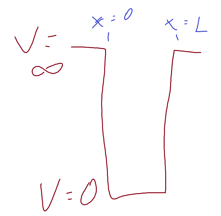
Infinite Square Well (Particle in a Box)

• V(x) has the form

  • V = 0 when \(0<x<L\)

  • V = \(\infty\) when \(x<0 \; or\; x>L\)

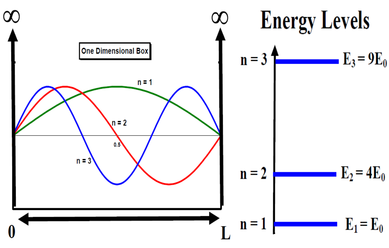
Infinite Square Well - Solutions

• Within the well, the Schrödinger Equation becomes:

\(- \frac{\hbar^2}{2m} \frac{d ^2 \psi}{d x^2} = E \psi\)

• General solution has the form

\(\psi = A cos(kx) + B\sin(kx)\)

• Where

\(k = \sqrt{\frac{2mE}{\hbar^2}}\)

ISW - Boundary Conditions

• Boundary conditions dictate \(\psi\) that vanishes at 0 and L

\(0 = A cos(k0) + B\sin(k0)\) \(0 = A cos(kL) + B\sin(kL)\)

• First condition must mean A=0

  • If A=0 then \(\sin(kL) = 0\) and \(k = n\pi /L\), n=1, 2, 3..
    • (not n = 0 because that would give \(\psi = 0\) everywhere)

• Means \(E_n = \frac{\hbar^2 \pi^2 n^2}{2mL^2}\)

• when we normalise we get

\(\psi_n = \sqrt{2/L} \sin(n\pi x /L)\)

Conjugated Dyes

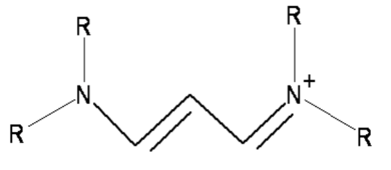
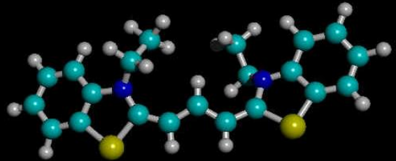
• Planar cations

• Number of carbons in chain varies

• End group (R) can be \(H\), \(CH_3\), etc

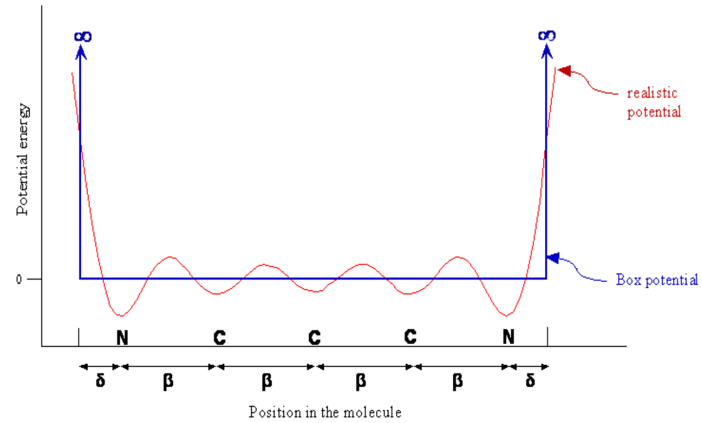
• Carbon chain acts like infinite square well

  • delocalised pi electrons over the length of the molecule between N ions
  • Free-Electron Molecular Orbital Model

• Potential looks like this:

• spectra looks like this:

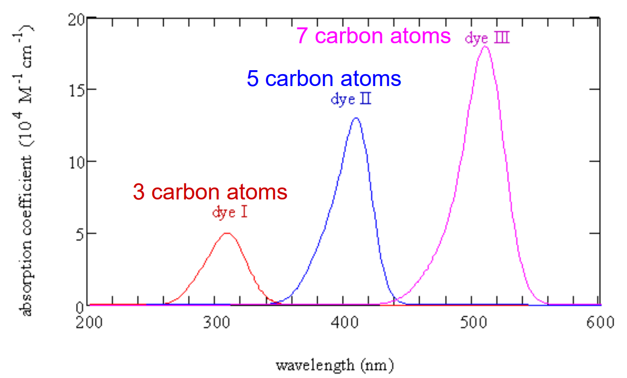
Spectra of Conjugated Dyes

• Absorption caused by transition from highest filled orbital (\(n_{HFO}\)) to lowest unfilled orbital (\(n_{LUO}\))

  • Get one electron from each carbon plus three from the nitrogens
  • N = (no of carbons) + 3

• \(n_{HFO} = N/2\) and \(n_{LUO} = N/2 + 1\) (Pauli Exclusion)

Remember \(E_n = \frac{\hbar^2 \pi^2 n^2}{2mL^2}\) for infinite square well \(\Delta E = E_{LUO} – E_{HFO} = \frac{\hbar^2 \pi^2n_{LUO}^2}{2mL^2} - \frac{\hbar^2 \pi^2n_{HFO}^2}{2mL^2}\)

\(\implies \Delta E = \frac{\hbar^2 \pi^2}{2mL^2} (n_{LUO}^2 - n_{HFO}^2)\)

\(\implies \Delta E = \frac{\hbar^2 \pi^2}{2mL^2} [(\frac{N}{2} + 1)^2 - (\frac{N}{2})^2]\)

\(\implies \Delta E = \frac{\hbar^2 \pi^2}{2mL^2} (N + 1)\)

\(\Delta E = 6.024 \times10^{-38} (N+1)/ L^2\)

taking \(h=6.626 \times 10^{-34}Js\) and \(m_e = 9.11 \times 10^{-31}kg\)

• \(\Delta E = 6.024 \times10^{-38} (N+1)/ L^2\)

• Application to dyes on slide 17 gives:

  • L for 3 carbons is 0.809nm
  • L for 5 carbons is 1.056nm
  • L for 7 carbons is 1.307nm

• Compares OK with C-C bond length of 0.146nm and C=C bond length of 0.134nm

• (remember \(E = \frac{hc}{\lambda}\))

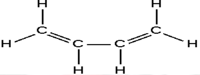
Spectrum of Butadiene

• Four carbon molecule

  • Four \(\pi\) electrons, N=4

  • Get \(\Delta E = \frac{\hbar^2 \pi^2 n^2}{2mL^2}(N+1) = \frac{5 \hbar^2 \pi^2}{2mL^2}\)

• Length of molecule is (two double bonds) + (one single bond) + (a bit more at each end, say a total of a single bond)

• This gives L = 0.56nm

• Then \(E = 9.61 \times 10^{-19}J\)

• And \(\lambda_{max}\) = 207nm

• Compares to experimental value of 210nm

• Got to admit agreement is pretty lucky, but still shows power of QM

Selection Rules for Square Well

• Not all transitions allowed, some have probability=0

• We’ll work out these selection rules for the infinite square well potential

• We’ll also show how longer molecules have stronger absorbtion

• Incident light causes transition from occupied level to higher previously unoccupied level

• Absorbs energy from light beam

• Strength of light-molecule interaction depends on electric dipole moment of molecule

  • \(\epsilon = - \mu .E\) where \(\mu\) is dipole moment

  • \(\mu = \Sigma x_i e_i\) where x is position and e is charge

• Light has long wavelength so E doesn’t depend on x

• In quantum mechanics, the transition dipole moment is given by:

\(\mu = \int \psi_f \;ex\; \psi_i dx\)

• When we evaluate this integral for the wavefunctions of the square well, we can see which ones disappear

• They disappear because integral = 0 because of symmetry

• These will be forbidden transitions

\(\mu = - \int_0^L \psi_{final} \; ex\; \psi_{initial}\; dx\)

\(\implies \mu = - \frac{2e}{L} \int_0^L x \sin(\frac{n_{final} \pi x}{L}) \; \sin(\frac{n_{initial} \pi x}{L})\; dx\)

• but \(\sin(x) \sin(y) = \frac{1}{2} [ \cos(x-y) - \cos(x+y)]\)

\(\implies \mu = - \frac{e}{L} \int_0^L x [\cos(\frac{ \pi x ( n_{final} - n_{initial})}{L}) \;- \; \cos(\frac{ \pi x ( n_{final} + n_{initial})}{L})]\; dx\)

• do this integration by parts using u = x and \(dv = \cos(x)dx\)

• gives \(\int_0^L x\; \cos(ax)\; dx = [\frac{x}{a} \sin(ax) + \frac{1}{a^2}\cos(ax)]_0^L\)

• then

\(\mu = - \frac{e}{L} (\frac{L}{\pi})^2[\frac{1}{n_{diff}^2}(\cos(n_{diff}\pi)-1) - \frac{1}{n_{total}^2}(\cos(n_{total}\pi)-1)\)

\(+ \frac{\pi}{n_{diff}} \sin(n_{diff}\pi) - \frac{\pi}{n_{total}} \sin(n_{total}\pi)]\)

where \(n_{diff} = n_{final} - n_{initial}\) and \(n_{total} = n_{final} + n_{initial}\)

See what happens when n is even or odd

• if n is even then \(\cos(n\pi) - 1 = 0\) and \(\sin(n\pi) = 0\)

\(\implies \mu = 0\) when \(n_{diff}\) is even and \(n_{total}\) is even

• this happens if both \(n_{initial}\) and \(n_{final}\) are both even or both odd

-on the other hand if one of \(n_{initial}\) and \(n_{final}\) is even and the other odd

\(\mu = \frac{2eL}{\pi^2}[\frac{1}{n_{diff}^2} - \frac{1}{n_{total}^2}]\)

• This all means:

  • No transition if initial and final state have same parity
    • i.e. both even or both odd
  • Transition if initial and final states have opposite parity
    • (\(n_{initial} – n_{final}\)) must be odd
  • Transition strength increases with L
    • Long molecules absorb strongly
    • See spectra on page 17

Equations

• \(i \hbar \frac{d T}{d t} = E \times T(t)\)
• \(T(t) = A e^{-iEt/\hbar}\)
• \(- \frac{\hbar^2}{2m} \frac{d ^2 \psi}{d x^2} + V(x) \psi = E \psi\)
• \(\psi_n = \sqrt{2/L} \sin(n\pi x /L)\)

• \(E_n = \frac{\hbar^2 \pi^2 n^2}{2mL^2}\)
• \(\Delta E = \frac{\hbar^2 \pi^2}{2mL^2} (N + 1)\)
• \(\mu = \frac{2eL}{\pi^2}[\frac{1}{n_{diff}^2} - \frac{1}{n_{total}^2}]\)

References

• Young & Freedman - chapter 40.2

• Serway & Jewett - chapter 7.4-7.8

• Krane - Modern Physics Chapter 5.4