06-Introduction to Quantum Physics

Physics Theory II PHYS2001

Summary

Light shows many properties consistent with its nature as being a wave; examples being difffraction and interference. But it also shows many properties that can only be explained by considering light as being a stream of particles, photons (\(\gamma\)). This conflict can be viewed as a wave-particle duality, with a photon as a probability wave.

Particles such as electrons also show similar effects.

The wave-like properties can be interpreted using Heisenberg’s Uncertainty Principle.

Wave Nature of Light
Particle Nature of Light
1. Blackbody Radiation & Planck
2. Photoelectric Effect
  - Energy & Momentum of Photons
3. Compton Effect
4. Pair Production

Mathematics of Wave Packets
Uncertainty Principle
Wave Nature of Particles
Equations
References

Wave Nature of Light

optical diffraction explained by waves
- analogous to phenomena in water waves, sound, etc
- \(\theta \propto \frac{\lambda}{d}\), d is aperture width

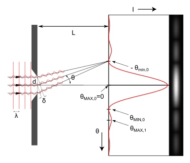
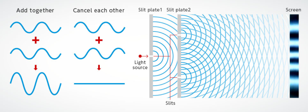
two-slit interference pattern (Young’s)
- \(n\lambda = d \times sin\theta\)

X-ray diffraction patterns we looked at last week also explained by wave nature of light

But there are problems

Blackbody Radiation
- classical model of the spectrum of thermal radiation (Rayleigh-Jeans) gives infinities at short wavelengths
- called ultraviolet catastrophy
- solved by Planck’s Radiation Law
photoelectric effect
Compton Scattering
Pair production

1. Blackbody Radiation

every object emits light because of its temperature
- hot bodies are brighter (Stefan Boltzman Law)
- hot bodies \(\implies\) more intense colours (Wien’s Displacement Law)
  - \(infrared \rightarrow crimson \rightarrow yellow \rightarrow blue \rightarrow uv\)

spectrum explained by Planck’s Radiation Law

\({\displaystyle u_{\lambda }(\lambda ,T)={\frac {8\pi hc}{\lambda ^{5}}}{\frac {1}{e^{hc/(\lambda k_{\mathrm {B} }T)}-1}}}\)

introduces Plank’s constant, \(h = 6.626 \times 10^{-34} Js\)
- also \(\hbar = \frac{h}{2\pi} = 1.055 \times 10^{-34} Js\)
- h is the talisman for quantum physics
where \(c = 2.99792458 \times 10^{8}m/s\) = speed of light
\(k_B = 1.380649 \times 10^{-23} J/K\) = Boltzman’s Constant

Equations for Our Photons

\(\omega = {2\pi}{f}\) = angular velocity
\(k = \frac{2\pi}{\lambda}\) = wave vector
\(p = \frac{h}{\lambda} = \hbar k\) = momentum
\(E_{\gamma} = hf = \hbar \omega\)
\(E_{\gamma} = \frac{hc}{\lambda} = \hbar k c = pc\)
also, photons are spin 1 particles \(\implies\) bosons

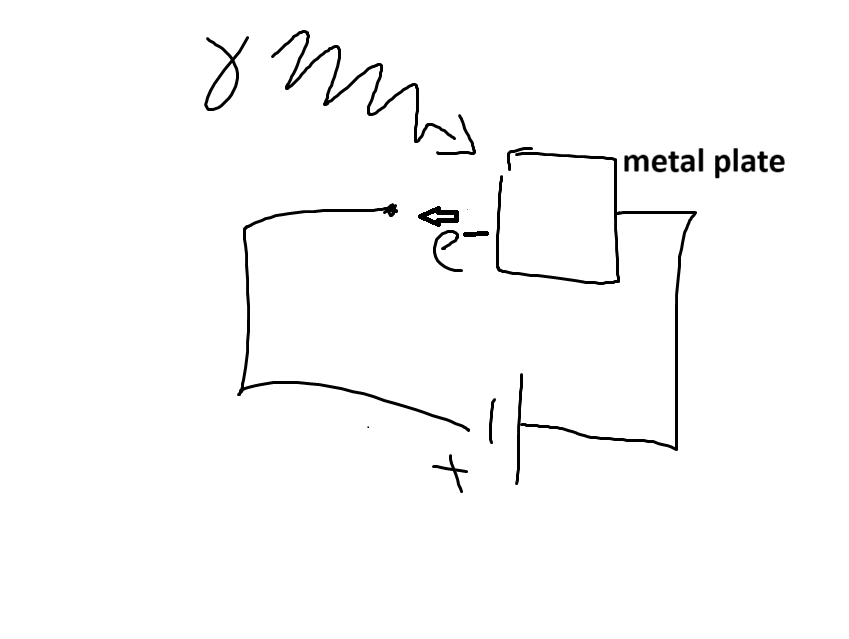
2. Photoelectric Effect

shine light on metal plate
electrons emitted
- would expect the brighter the light \(\implies\) the stronger the electric field \(\implies\) the more energetic the electrons leaving plate
don’t see this
- energy of electrons depends on light wavelength
- number of electrons depends on brightness
- \(KE_{{max}_{e^-}} = hf - \phi\)

adjust voltage until just strong enough to stop all electrons
- \(eV = hf - \phi\)

3. Compton Effect

if light is just a wave, scattering off particles won’t effect \(\lambda\)
but we do see change in \(\lambda\)
- have to look pretty carefully
- works best for x-rays scattering off electrons
get \(\Delta \lambda = \lambda - \lambda_0 = \frac{h}{mc}(1-cos \theta)\)

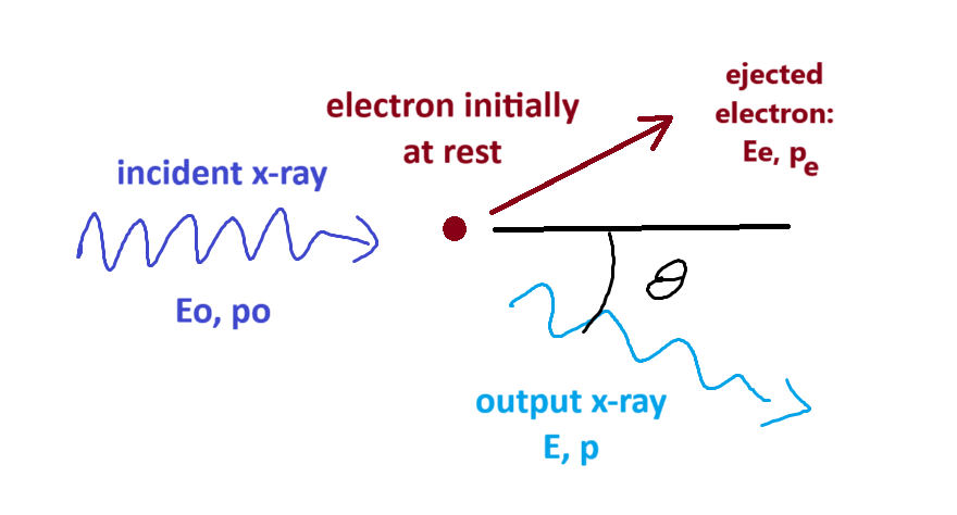
energy before = energy after

\(mc^2 + E_o = E_e + E\) \(\implies E_e = E_0 + mc^2 - E\) \(\implies \sqrt{(mc^2)^2+ (p_ec)^2}\) \(= p_oc + mc^2 - pc\) \(\implies \sqrt{(mc)^2+ (p_e)^2}\) \(= p_o + mc - p\)

conservation of momentum

\(\vec{p_0} = \vec{p} + \vec{p_e}\) \(\implies \vec{p_e} = \vec{p_0} - \vec{p}\) \(\implies p_e^2 = (\vec{p_0} - \vec{p})\cdot(\vec{p_0} - \vec{p})\) \(\implies p_e^2 = p_0^2 + p^2 - 2p_0 p\; cos\theta\)

combining, replacing \(p_e^2\) from energy equation

\((mc)^2 + p_0^2 + p^2 - 2p p_0 cos \theta\) \(= p_0^2 + p^2 -2pp_0 + m^2c^2 + 2p_0mc - 2pmc\)

lots of terms cancel

\(-2pp_0 cos \theta = -2p_0p + 2mc(p_0-p)\)

\(p_0p(1-cos\theta) = mc(p_0-p)\) \(\frac{1}{mc}(1-cos\theta) = \frac{1}{p}- \frac{1}{p_0}\)

Compton Shift is Pretty Small

photons scattering off electrons at \(\theta = 80 ^{\circ}\)
\(\Delta \lambda = \frac{h}{mc} (1 - cos\theta)\)
\(= \frac{6.626 \times 10^{-34}}{9.11 \times 10^{-31} \;\times \; 3 \times 10^8}\; \times (1-cos 80^{\circ})\)
\(= 2.426 \times 10^{-12} \; \times \; (1 - 0.1736)\)
\(= 2.005 \times 10^{-12} m\)
\(= 0.002005 \; nm\)

gets worse if x-ray doesn’t liberate electron
- replace \(m = 9.11 \times 10^{-31} kg\) by mass of atom

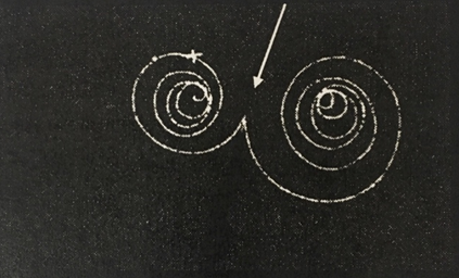
4. Pair Production

Mathematics of Waves

single wave \(A = A_0 sin(kx - \omega t)\)
- (neat way of expressing this \(A = e^{i(kx - \omega t)}\))
- solution to equation \(\frac{\partial^2A}{\partial t^2}-(\frac{\omega}{k})^2 \frac{\partial^2A}{\partial x^2} = 0\)
- angular velocity; \(\omega = 2 \pi f\), where f is the frequency
- wavenumber; \(k = \frac{2 \pi}{\lambda}\), where \(\lambda\) is the wavelength
- using \(v = f\lambda\) get \(v = \frac{\omega}{k}\)
- (this is the phase velocity, \(v_p\))

Add Two Waves of Slightly Different Frequency Together

\(A(x, t) = A_0 sin[(k-\Delta k)x - (\omega - \Delta \omega) t] +\) \(A_0 sin[(k+\Delta k)x - (\omega + \Delta \omega) t]\)
rearranging
\(A(x, t) = A_0 sin[(kx-\omega t) - (\Delta kx - \Delta \omega t)] +\) \(A_0 sin[(kx-\omega t) + (\Delta kx - \Delta \omega t)]\)
like adding two sines: \(sin(A+B) + sin(A-B) = 2sin(A)cos(B)\)
get: \(A(x, t) = 2 \times A_0 sin(kx - \omega t)\; cos(\Delta kx - \Delta \omega t)\)
a sine wave modulated by a much slower cosine wave

\(A(x, t) = 2 \times A_0 sin(kx - \omega t)\; cos(\Delta kx - \Delta \omega t)\)
The sine wave has velocity \(v_p = \omega / k\)
The longer cosine wave modulating it has velocity \(v_g = \Delta \omega / \Delta k\)
this last we call the Group Velocity

Example

Add the two waves \(A_0 sin(k_1x - \omega_1 t)\) and \(A_0 sin(k_2x - \omega_2 t)\) where \(k_1 = 6.4 \; rads/m\), \(\omega_1 = 9.2 \; rads/s\), \(k_2 = 6.0 \; rads/m\), and \(\omega_2 = 9.0 \; rads/s\)
the phase velocity is \(\omega / k\) where \(\omega = \frac{(\omega_1 + \omega_2)}{2}\) and \(k = \frac{(k_1 + k_2)}{2}\) giving \(v_p = 9.1 / 6.2 = 1.47 m/s\)
the group velocity is \(\Delta \omega / \Delta k\) where \(\Delta \omega = \frac{(\omega_1 - \omega_2)}{2}\) and \(\Delta k = \frac{(k_1 - k_2)}{2}\) giving \(v_g = 0.2 / 0.4 = 0.50 m/s\)

Adding More than Two Waves

the two wave example above gives the general principle, but in practice many more waves combine to form a wave packet
- they’ll all have closely spaced frequencies (\(\frac{\omega}{2\pi}\))
- and closely spaced wavenumbers, k
the average values for \(\omega\) and k will generate the phase velocity
the way in which \(\omega\) and k change across the wavepacket, \(d \omega / dk\), will give the group velocity
the group velocity is of greater physical significance

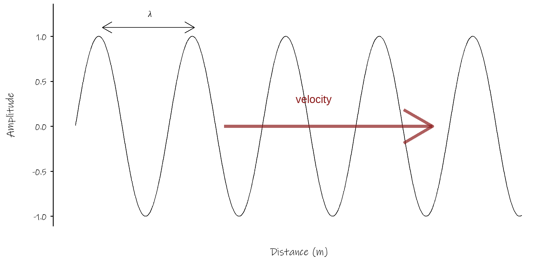
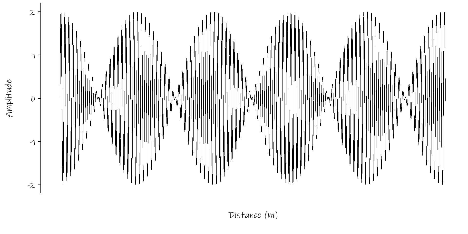
Wavepacket of 500 Sine Waves

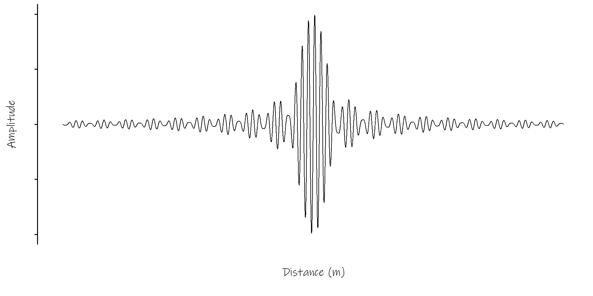
Credit: Institute of Sound and Vibration Research

Heisenberg’s Uncertainty Principle

light diffraction can be though of as an illustration of the uncertainty principle
slit width \(d\) so therefore uncertainty in photon position of \(\Delta x = d\)
width of diffraction pattern = \(\Delta \theta = \frac{\lambda}{d}\)
- range of momentum values = \(\Delta p = p \Delta \theta = p \frac{\lambda}{d}\)
- but \(p = \frac{h}{\lambda}\)
- substituting we get \(\Delta p = \frac{h}{\lambda} \frac{\lambda}{d} = \frac{h}{d}\)
- but \(\Delta x = d\), so \(\Delta p = \frac{h}{\Delta x}\)
- \(\implies \Delta x \Delta p \ge h\)

Wave Nature of Other Stuff

electrons fired through a double slit apparatus also show a diffraction / interference pattern
- Davison Germer experiment with beam of electrons at nickel plate
- even when we dial the intensity way down, one electron at a time, we see the same pattern
- and this is also true for light, one photon at a time

we have \(E = \hbar \omega\)
for mass particles we have \(E = \frac{1}{2} m v^2 = \frac{p^2}{2m}\)
We need a differential equation that can work with the equation for a plane wave and yet give us the correct for the relation between energy and momentum
- Need to be proportional to \(k^2\), not \(k\)
- How about differentiating twice on t but just once on x?

something like \(\frac{\partial A}{\partial t} = \propto \frac{\partial^2A}{\partial x^2}\)
or, replacing \(A\) with \(\Psi\): \(\frac{\partial \Psi}{\partial t} = \propto \frac{\partial^2 \Psi}{\partial x^2}\)
if we put in the plan wave solution, \(\Psi = e^{i(kx-\omega t)}\) get
\(-k^2 = i \propto \omega\)
if we use \(p = \hbar k\) and \(E = \frac{p^2}{2m}\) get:
- \(\propto = -2mi/\hbar\)
- feed this back in to our equation and rearrange to get:

\(i \hbar \frac{\partial \Psi}{\partial t} = - \frac{\hbar^2}{2m} \frac{\partial ^2 \Psi}{\partial x^2}\)

this is in free space, no forces
if we add a potential, \(V\), we get

\(\; \; i \hbar \frac{\partial \Psi}{\partial t} = - \frac{\hbar^2}{2m} \frac{\partial ^2 \Psi}{\partial x^2} + V\Psi\)

Equations

\(A = A_0 sin(kx - \omega t)\)
\(A = e^{i(kx - \omega t)}\))
\(\frac{\partial^2A}{\partial t^2}-(\frac{\omega}{k})^2 \frac{\partial^2A}{\partial x^2} = 0\)
\(\omega = 2 \pi f\)
\(k = \frac{2 \pi}{\lambda}\)

\(v = \frac{\omega}{k}\)
\(p = \frac{h}{\lambda} = \hbar k\)
\(E = hf = \frac{hc}{\lambda}= \hbar c k\)
\(v_p = \omega / k\)
\(v_g = \partial \omega / \partial k\)
\(\Delta \lambda = \frac{h}{mc} (1 - cos \theta)\)